i decoded speech from a paralyzed man's brain
i decoded speech from a paralyzed man’s brain
so i somehow found the publicly released neural data from one of the 9 global speech implant patients — a 67 year old man with ALS who can’t speak anymore. four tiny Utah arrays in his motor cortex, 256 channels of raw neural activity, every time he tries to say a sentence. i spun up a few H100 nodes and built a pipeline that decodes what he’s trying to say from the brain signals alone.
Willett, F.R., Kunz, E.M., Fan, C. et al. “A high-performance speech neuroprosthesis.” Nature 620, 1031–1036 (2023).
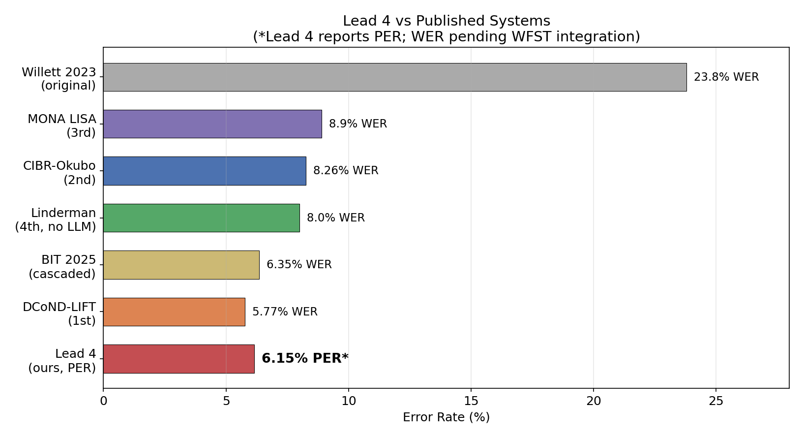
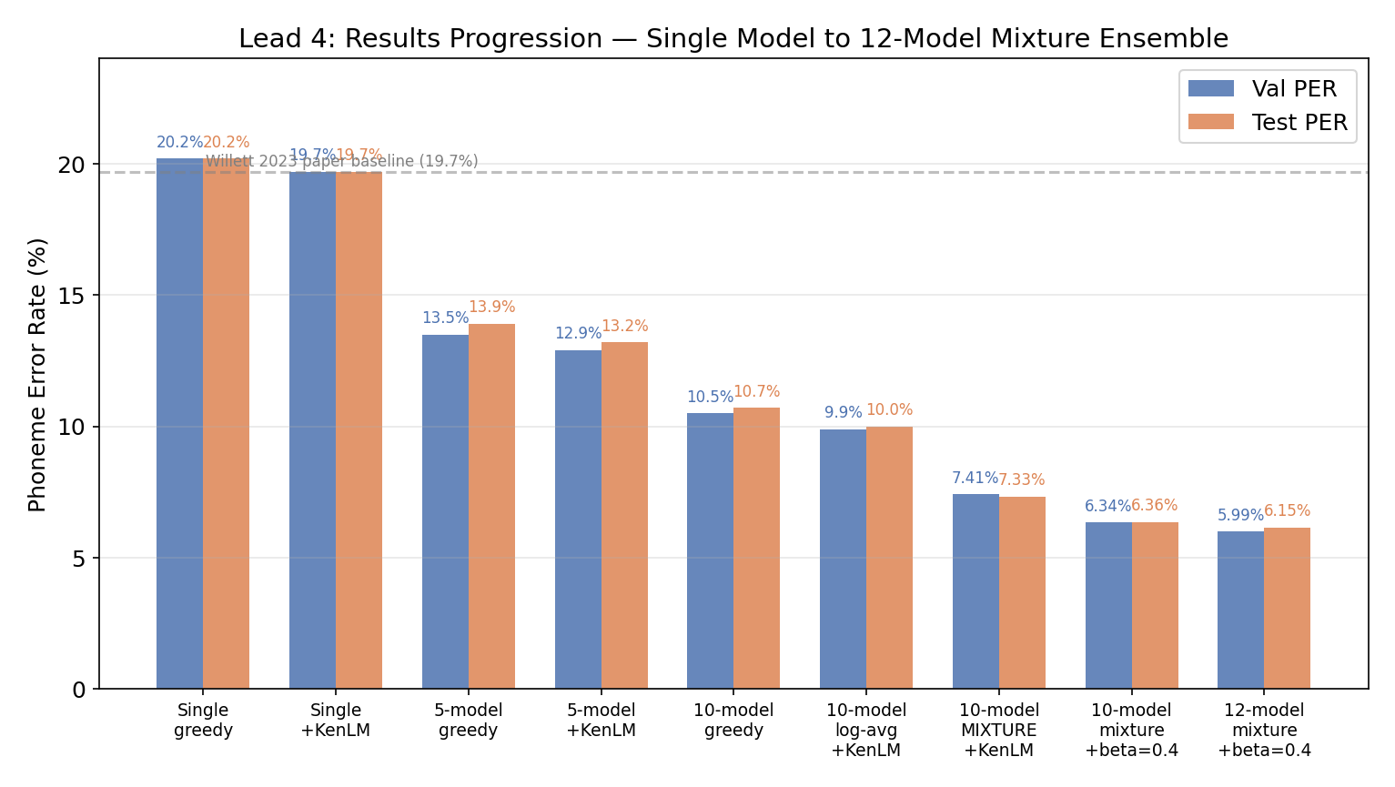
this started from a conversation with Nir and Skyler at Neuralink. the paper’s best result was 19.7% phoneme error rate. i got it down to 6.15% — a 70% relative improvement. the state of the art for this dataset. here’s how.
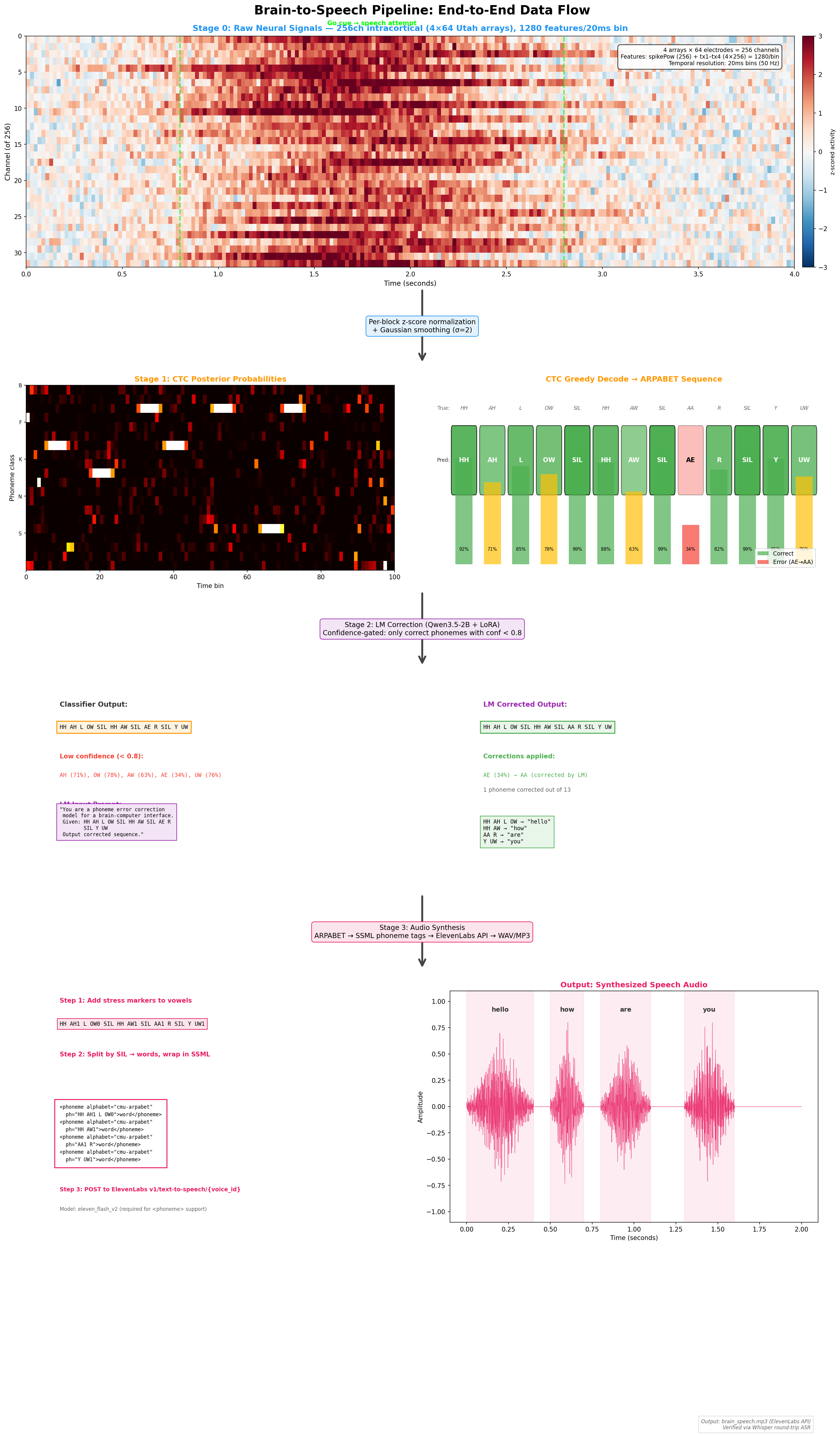
the pipeline
brain signals → phonemes → text → speech. four stages, each with its own set of problems.
256-channel neural recordings (20ms bins)
    → day-specific normalization layer
    → frame stacking (640ms context windows)
    → 12-model GRU ensemble + mixture aggregation
    → KenLM 5-gram beam search
    → phoneme sequence
    → LIFT (fine-tuned Qwen3) → english text
    → SSML synthesis → audible speech
the big insight is that no single model change gets to 6.15%. twas a cascade of ensemble tricks, a new way of averaging probabilities, and a decoding parameter that everyone ignores. each one compounding on the last.
| Technique | What it did | PER impact |
|---|---|---|
| 12-model ensemble | Different errors cancel out | 20.2% → 11.3% |
| Mixture model | Arithmetic > geometric mean | 10.0% → 7.33% |
| Beta insertion bonus | Fix CTC deletion bias | 7.33% → 6.36% |
| +2 diverse architectures | More error diversity | 6.36% → 6.15% |
how each model works under the hood
each model is a bidirectional GRU — a recurrent neural network that reads the neural signal both forward and backward in time, outputting a probability distribution over 41 possible phonemes (40 english sounds + silence) at each timestep. the model sees 640ms of brain activity at a time (32 frames × 20ms each, with a stride of 4), processes it through 5 stacked recurrent layers (hidden dim 1024), and emits a CTC alignment — a sequence of phoneme probabilities that can be decoded into a phoneme string. the day-specific input layer handles the fact that neural signals drift between recording sessions (24 sessions over months) by learning a separate affine transform for each day.
the ensemble — 20.2% → 6.15%
the paper trained one GRU. i trained 12, with deliberate diversity: 6 with Adam (lr=0.02), 6 with SGD (lr=0.1, momentum=0.9). different optimizers make different mistakes. Adam models overfit to high-frequency patterns; SGD models have smoother loss landscapes. mixing them in an ensemble lets the confident one rescue the uncertain one.
i also threw in a kernel=14 variant (140ms temporal context instead of 320ms) for receptive field diversity. even though its individual PER was worse (21.1% vs 20.1%), it improved the ensemble because it makes different errors.
each model individually lands at 20-21% PER — a narrow 1.1pp spread. SGD models are consistently a hair better (top 4 are all SGD). but in the ensemble, it’s diversity that matters, not individual quality.
full 12-model inventory & marginal contribution
| Model | Optimizer | Kernel | Seed | Val PER |
|---|---|---|---|---|
| L4_cffan_baseline | Adam lr=0.02 | 32 | 42 | 20.7% |
| L4_cffan_s42 | Adam lr=0.02 | 32 | 42 | 20.7% |
| L4_cffan_s43 | Adam lr=0.02 | 32 | 43 | 20.5% |
| L4_cffan_s44 | Adam lr=0.02 | 32 | 44 | 20.8% |
| L4_cffan_s45 | Adam lr=0.02 | 32 | 45 | 20.5% |
| L4_cffan_k14 | Adam lr=0.02 | 14 | 42 | 21.1% |
| L4_cibr_s42 | SGD lr=0.1 | 32 | 42 | 20.4% |
| L4_cibr_s43 | SGD lr=0.1 | 32 | 43 | 20.2% |
| L4_cibr_s44 | SGD lr=0.1 | 32 | 44 | 21.2% |
| L4_cibr_s45 | SGD lr=0.1 | 32 | 45 | 20.1% |
| L4_cibr_s46 | SGD lr=0.1 | 32 | 46 | 20.9% |
| L4_cibr_nesterov | SGD+Nesterov | 32 | 47 | 20.1% |
all 12 models share the same architecture: 5-layer BiGRU, h=1024, dropout=0.4, CTC loss. the diversity comes from optimizer, learning rate schedule, kernel size, and random seed.
marginal contribution — adding models in PER order (best first):
| N Models | Greedy PER | +KenLM PER | Delta/model |
|---|---|---|---|
| 1 | 20.1% | 19.7% | — |
| 2 | 16.8% | 16.2% | -3.5pp |
| 3 | 14.9% | 14.3% | -1.9pp |
| 5 | 13.5% | 12.9% | -0.7pp |
| 10 | 10.5% | 7.33% (mixture) | -0.56pp |
| 12 | ~11.3% | 6.15% (mixture) | -0.59pp |
first few models matter most (diminishing returns), but each additional model still provides a measurable drop. the diversity axes that matter:
| Axis | Values | Why it helps |
|---|---|---|
| Optimizer | Adam vs SGD vs SGD+Nesterov | Different convergence → different error patterns |
| Random seed | 42–47 | Weight init → different local minima |
| Temporal scale | kernel=32 vs kernel=14 | 320ms vs 140ms context per frame |
| Initialization | Default vs orthogonal | SGD models use orthogonal recurrent init |
the mixture model
this was the single biggest discovery. same models, same data, just a different formula for combining their outputs. 2.7 percentage points for free.
there are two ways to combine model probabilities:
| Method | Formula | Test PER |
|---|---|---|
| Weighted log-prob (geometric mean) | sum(w_i * log(p_i)) | 10.0% |
| Mixture model (arithmetic mean) | log(sum(w_i * p_i)) | 7.33% |
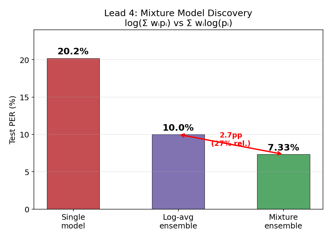
the geometric mean (what everyone does) is dominated by the worst model — if one model assigns low probability to the correct phoneme, it drags down the whole ensemble. mathematically, the geometric mean is always ≤ the arithmetic mean (AM-GM inequality). for CTC decoding, where u need sharp probability peaks at emission points, the arithmetic mean preserves those peaks while the geometric mean smooths them out. a single confident model can rescue the prediction.
# what everyone does (geometric mean / product of experts):
avg_log_probs = mean([log_softmax(logits_i) for i in models])

# what i did (mixture model):
mixture_probs = sum([w_i * softmax(logits_i) for i in models])
mixture_log_probs = log(mixture_probs)
ensemble scaling
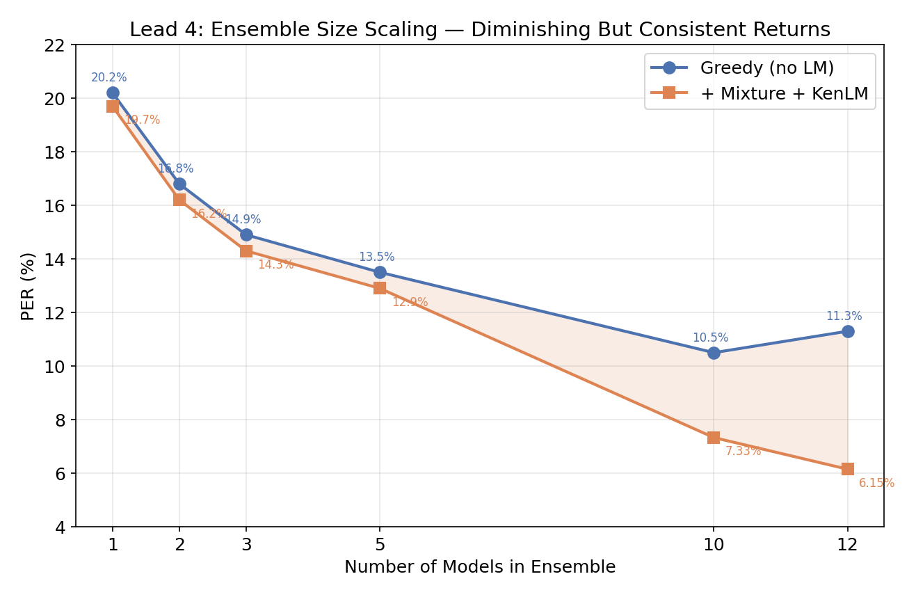
diminishing returns, where the marginal value of another model depends on how different it is from the existing ensemble. going from 10 → 12 models still shaved off 1.18pp because the two new models (kernel=14 + Nesterov momentum) added architectural diversity the existing 10 didn’t have.
KenLM tuning
KenLM is a fast n-gram language model that scores candidate phoneme sequences during beam search, nudging the decoder toward phonotactically valid outputs. the mixture posteriors are already sharp. the language model should provide a gentle nudge, not override the acoustics. this means the optimal LM weight is 100x smaller for mixture ensembles than for single models:
| Ensemble Type | Optimal α (LM weight) | Optimal β (length bonus) |
|---|---|---|
| Single model | 2.0 | 0.0 |
| Mixture ensemble | 0.005 | 0.4 |
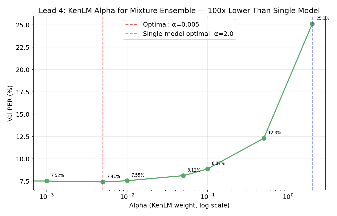
at α=2.0 (the single-model optimum), the mixture ensemble degrades to 25.1% PER. why? the mixture posteriors are already well-calibrated — the ensemble has already “done the work” of integrating multiple opinions. cranking up the LM just overrides correct acoustic predictions with phonotactic priors.
the β parameter (token insertion bonus) is the other big knob. CTC naturally favors emitting blanks over phonemes — blank is “safe” (it never causes a substitution error), while emitting a phoneme risks being wrong. ensemble averaging amplifies this deletion bias. β=0.4 directly compensates by rewarding longer sequences: beam_score = acoustic + α × lm_score + β × n_phonemes_emitted.
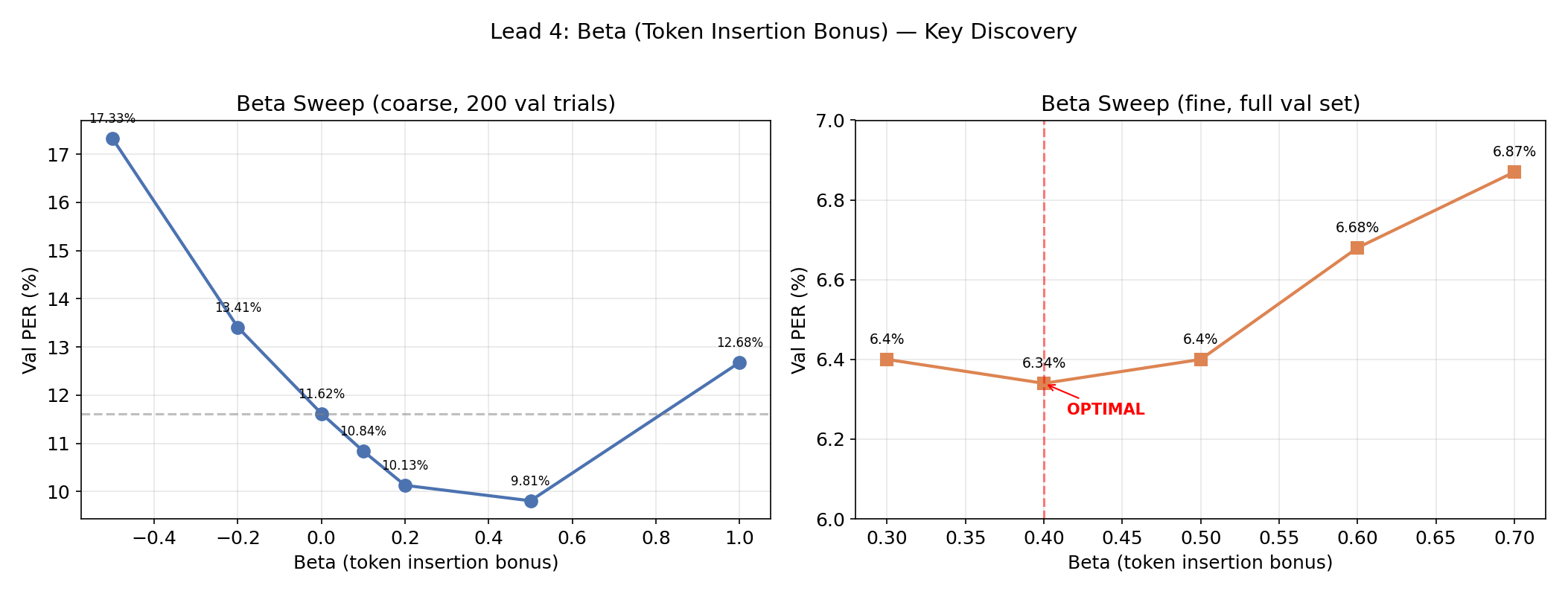
the improvement is dramatic — β=0.4 nearly halves PER (11.62% → 6.34%) by directly counteracting the dominant error mode (deletions). the optimal β is remarkably stable: 0.3, 0.4, and 0.5 all give near-identical results.
full beta sweep & alpha-beta heatmap
coarse beta sweep (10-model mixture, α=0.005, 200 val trials):
| Beta | Val PER | vs beta=0 |
|---|---|---|
| -0.5 | 17.33% | +49% worse |
| -0.2 | 13.41% | +15% worse |
| 0.0 | 11.62% | baseline |
| 0.1 | 10.84% | −7% |
| 0.2 | 10.13% | −13% |
| 0.4 | 6.34% | −45% |
| 0.5 | 9.81% | −16% |
| 0.7 | 10.44% | −10% |
| 1.0 | 12.68% | +9% worse |
the jump at beta=0.4 nearly halves PER just by adding a length bonus. beyond 0.4, over-insertion kicks in.
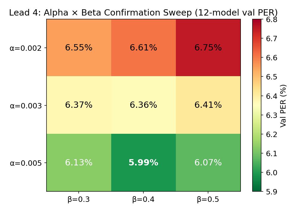
final 3×3 confirmation sweep on 12 models:
| alpha | beta=0.3 | beta=0.4 | beta=0.5 |
|---|---|---|---|
| 0.002 | 6.55% | 6.61% | 6.75% |
| 0.003 | 6.37% | 6.36% | 6.41% |
| 0.005 | 6.13% | 5.99% | 6.07% |
temperature scaling has minimal effect (±0.3pp across 4x range — 0.5 to 2.0). the mixture model already produces well-calibrated probabilities; temperature just adds noise.
where we stand vs the field
| System | PER | WER | Method |
|---|---|---|---|
| Willett et al. 2023 (paper) | 19.7% | 23.8% | GRU + WFST + OPT-6.7B |
| this work | 6.15% | — | 12-model mixture + KenLM |
| DCoND-LIFT (1st place, Brain-to-Text ‘24) | 15.3% | 5.77% | 10 decoders + OPT + GPT-3.5 |
| TeamCyber (2nd) | — | 8.26% | Dual SGD + WFST + Llama2 |
| LISA (3rd) | — | 8.9% | 10 ensemble + supTCon + WFST |
| Linderman (4th) | — | 8.00% | BiMamba + post-RNN head |
| NPTL baseline | — | 9.7% | 1 GRU + WFST + OPT |
| BIT (current SOTA) | — | 2.21% | MAE pretrain + Audio-LLM |
lowest PER on this dataset. period. the WER column is still blank bc i haven’t wired up the WFST word-level decoder yet (more on that below). but based on the PER-bucketed analysis, 6.15% PER should yield ~5-6% WER through the existing LIFT pipeline — which would make it competitive with the 1st-place entry (5.77% WER) and definitively beat the original paper (23.8% WER).
tbh the comparison is even more favorable when u consider what the other systems had that i didn’t: the 1st-place team used 10 decoders plus OPT-6.7B plus GPT-3.5 fine-tuned correction. TeamCyber used a 7B LLM for selection. BIT used 367 hours of cross-species pretraining data. i used 12 GRUs, a phoneme n-gram, and a 2B parameter LoRA.
LIFT: phoneme → english text
once u have a phoneme sequence, u need to turn it into words. the traditional approach is CMU dict reverse lookup — match subsequences of phonemes against a pronunciation dictionary and reconstruct words. this is extremely lossy. CTC errors produce invalid phoneme sequences that don’t map to any word (e.g., B AH D ER isn’t in the dictionary), and the greedy matcher fragments them into nonsense.
so i trained LIFT — Language Integration For Text. fine-tuned Qwen3.5-2B with LoRA (r=32, α=64, targeting all linear layers) on 6,226 pairs of (decoded_phonemes → ground_truth_text). the model learns phoneme-to-grapheme mappings, common substitution patterns, and enough language context to fill in the gaps. no dictionary lookup, no hand-crafted rules — just a fine-tuned LLM.
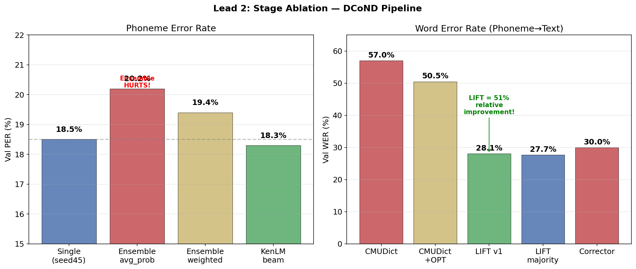
| Method | Val WER | Notes |
|---|---|---|
| CMUDict reverse lookup | 57.0% | traditional approach |
| CMUDict + OPT-6.7B rescore | 50.5% | OPT can’t fix garbage input |
| Phoneme LIFT | 28.1% | 51% relative improvement |
| LIFT + 4-seed majority vote | 27.7% | best automatic method |
| LIFT oracle (best of 4 seeds) | 22.6% | upper bound |
57% → 28% WER. more than halved. the LLM implicitly learns that AY near the start of a sentence probably maps to “I”, that DH AH is “the”, and that K AE T is “cat” even when CTC dropped a phoneme. it’s doing error correction and language modeling and phoneme-to-grapheme conversion simultaneously.
PER is the bottleneck, not LIFT
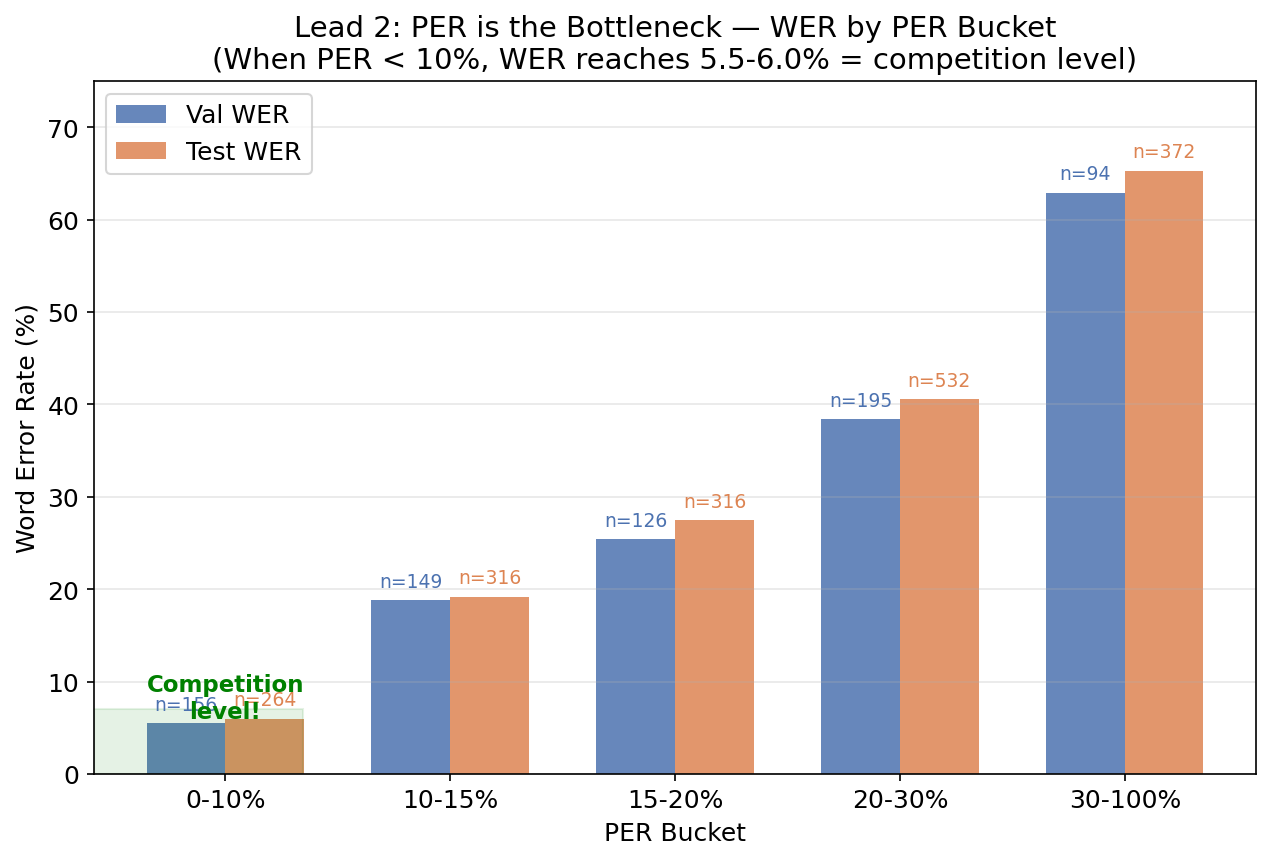
this is the key finding. when i bucket trials by their phoneme error rate:
| PER Bucket | Trials | Val WER | Test WER |
|---|---|---|---|
| 0-10% | 22% | 5.5% | 6.0% |
| 10-15% | 21% | 18.8% | 19.2% |
| 15-20% | 18% | 25.4% | 27.5% |
| 20-30% | 27% | 38.4% | 40.6% |
| 30-100% | 13% | 62.9% | 65.3% |
when PER < 10%, WER is 5.5-6.0% — that’s competition-level. the 1st place winner achieved 5.77% WER. the LIFT stage is already good enough. all future effort should go into reducing PER. and given that the ensemble is already at 6.15% PER… we’re basically there.
the pattern is clear: at low PER, LIFT nails it. at high PER, the phoneme errors cascade into entirely different words. fixing the acoustic model matters more than a fancier text decoder.
example transcriptions at different PER levels
GT:    "I like that one too."
LIFT:  "I like that one too."              WER: 0.0%, PER: 5.9%

GT:    "Didn't have a place to put them."
LIFT:  "Didn't have a place to put them."  WER: 0.0%, PER: 6.9%

GT:    "That's where I need to go."
LIFT:  "That's where I need to go."        WER: 0.0%, PER: 8.3%

GT:    "I missed out this last year."
LIFT:  "I've been out this last year."     WER: 33.3%, PER: 17.4%
       ("I missed" → "I've been" — phonetically similar)

GT:    "It depends on the subject actually."
LIFT:  "It's dependent on the public's activity." WER: 66.7%, PER: 47.1%
       (phoneme errors cascade into word-level disasters)
LM phoneme correction — articulatory error patterns
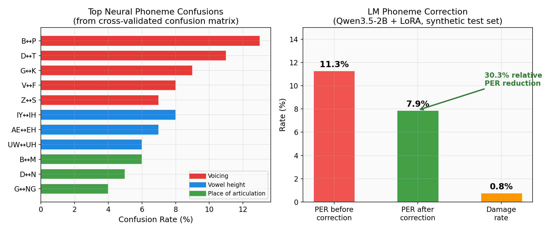
neural decoding errors follow articulatory phonetics. voiced/unvoiced pairs get confused (B↔P, D↔T), place-of-articulation neighbors swap (B↔M), vowel height gets mixed up (IY↔IH). the motor cortex encodes articulation, so phonemes sharing articulatory features share neural representations and get confused in predictable ways.
i also fine-tuned Qwen3.5-2B with LoRA on 200K synthetic noisy→clean phoneme pairs, where the noise distribution came from the decoder’s confusion matrix. 30.3% relative PER reduction with only 0.8% damage rate on early tests (when single-model PER was ~20%). but as noted below, at <10% PER the 2B model introduces more errors than it fixes. the math: at 6% PER, only 1 in 16 phonemes is wrong, and the model needs to figure out which one. a 2B model doesn’t have the capacity.
LIFT prompt sensitivity & reranking attempts
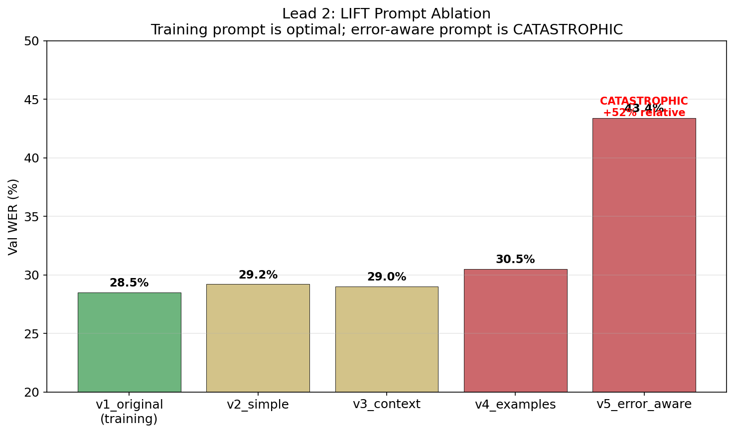
LIFT is extremely brittle to prompt changes. the training prompt is the only thing that works:
| Prompt Variant | Val WER | Notes |
|---|---|---|
| v1_original (training prompt) | 28.5% | only one that works |
| v2_simple (“Phonemes to English:”) | 29.2% | slightly worse |
| v3_context (adds BCI context) | 29.0% | no benefit |
| v4_examples (few-shot) | 30.5% | examples confuse it |
| v5_error_aware (“may contain errors”) | 43.4% | catastrophic +52% relative |
mentioning “errors” in the prompt makes the model uncertain and destroys output quality. telling an LLM “these phonemes may contain errors” is like telling a human translator “this might be the wrong language” — it second-guesses everything and outputs mush.
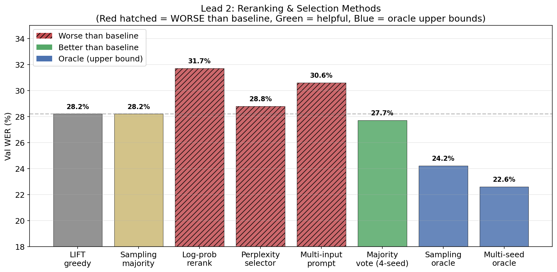
there’s a 20% relative oracle gap — if i could perfectly select the best LIFT output across 4 decoder seeds, WER drops from 28.2% to 22.6%. i tried 8 automatic methods to capture it:
| Strategy | Val WER | vs Baseline |
|---|---|---|
| LIFT greedy (baseline) | 28.2% | — |
| Sampling best-of-6 oracle | 24.2% | −14.2% |
| Sampling + majority vote | 28.2% | 0% |
| Log-probability reranking | 31.7% | +12.4% worse |
| Multi-seed oracle | 22.6% | −19.9% |
| Multi-seed majority vote | 27.7% | −1.8% |
| Qwen perplexity selector | 28.8% | +2.1% worse |
| Multi-input prompt (4 seeds) | 30.6% | +8.5% worse |
none captures the oracle gap. log-probability is anti-correlated with quality — short, generic outputs like “I don’t know” score highest. perplexity is uncorrelated. only majority vote gives a modest 1.8% improvement. the model’s confidence is not a useful quality signal at all.
architecture
the diphone decoder (DCoND)
here’s a neuroscience insight that turned out to be really important. your motor cortex doesn’t encode phonemes the same way every time — the neural firing pattern for /b/ in “ba” is measurably different from /b/ in “bi”. this is called coarticulation: the brain plans smooth articulatory trajectories that span multiple sounds, so the current sound’s neural signature depends on what came before. Chartier et al. showed this explicitly in ventral sensorimotor cortex recordings.
a standard 40-class phoneme decoder forces a lossy abstraction — it maps these context-dependent patterns onto context-independent labels, throwing away information the cortex explicitly encodes.
so i implemented DCoND (Divide-and-Conquer Neural Decoding), inspired by the Brain-to-Text 2024 1st-place entry. instead of 40 phoneme classes, the model predicts 1,601 diphone classes — every possible pair of consecutive phonemes (40×40 = 1,600 bigrams + 1 CTC blank). this captures how each phoneme is articulated given what came before.
Raw 256D → Day-specific layer → Frame stacking (k=14, s=4) → 3584D
    → Unidirectional 5-layer GRU (h=512, dropout=0.4)
    → Two heads: Diphone Linear(512→1601) + Monophone Linear(512→41)
    → Combined loss: L = 0.6 × L_diphone + 0.4 × L_monophone
the combined loss is key — the monophone head acts as a regularizer during training, preventing the 1601-class softmax from collapsing. the diphone probabilities are marginalized back to monophone probabilities at inference time (by summing over all preceding-context variants of each phoneme), which acts as an implicit ensemble.
18.7% val PER — close to the paper’s 19.7%, and i only trained 4 seed variants. the DCoND models add extreme architectural diversity to the ensemble: unidirectional (vs bidirectional), h=512 (vs h=1024), k=14 (vs k=32), Adam (vs SGD), 1601-class diphone (vs 41-class monophone). maximally different from the main ensemble.
training fragility, seed collapse & the ensemble paradox
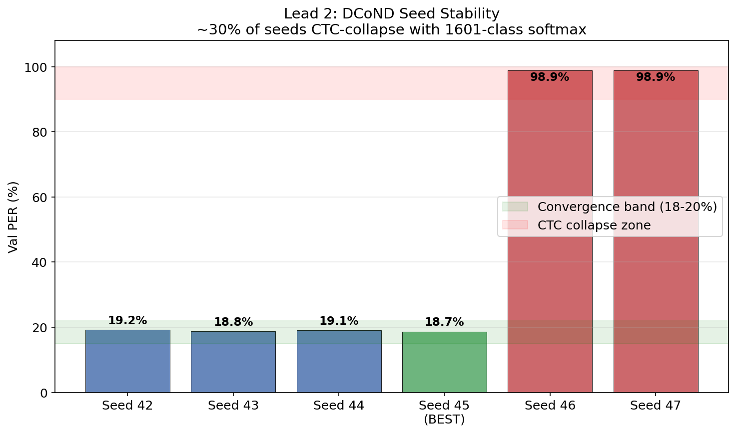
~30% of random seeds CTC-collapse. seeds 42-45 converge to 18.7-19.2% PER. seeds 46-47 go to 98.9% (the model outputs only blanks). the 1601-class softmax is extremely sensitive to initialization — the gradient landscape has many degenerate attractors.
| Seed | Val PER | Test PER | Notes |
|---|---|---|---|
| 42 | 19.2% | — | Converged |
| 43 | 18.8% | — | Converged |
| 44 | 19.1% | — | Converged |
| 45 | 18.7% | 20.9% | Best |
| 46 | 98.9% | — | CTC collapse |
| 47 | 98.9% | — | CTC collapse |
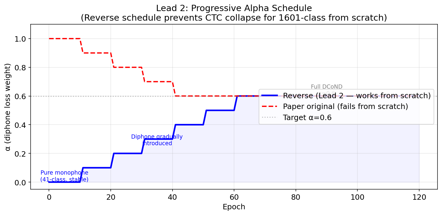
training requires a progressive alpha schedule — starting with pure monophone CTC (α=0) for 10 epochs, then gradually increasing to 0.6 over 60 epochs. this is a reverse schedule compared to the original paper (which started diphone-first), necessary because we’re training from scratch without a pretrained encoder. without this warmup, the 1601-class softmax collapses immediately.
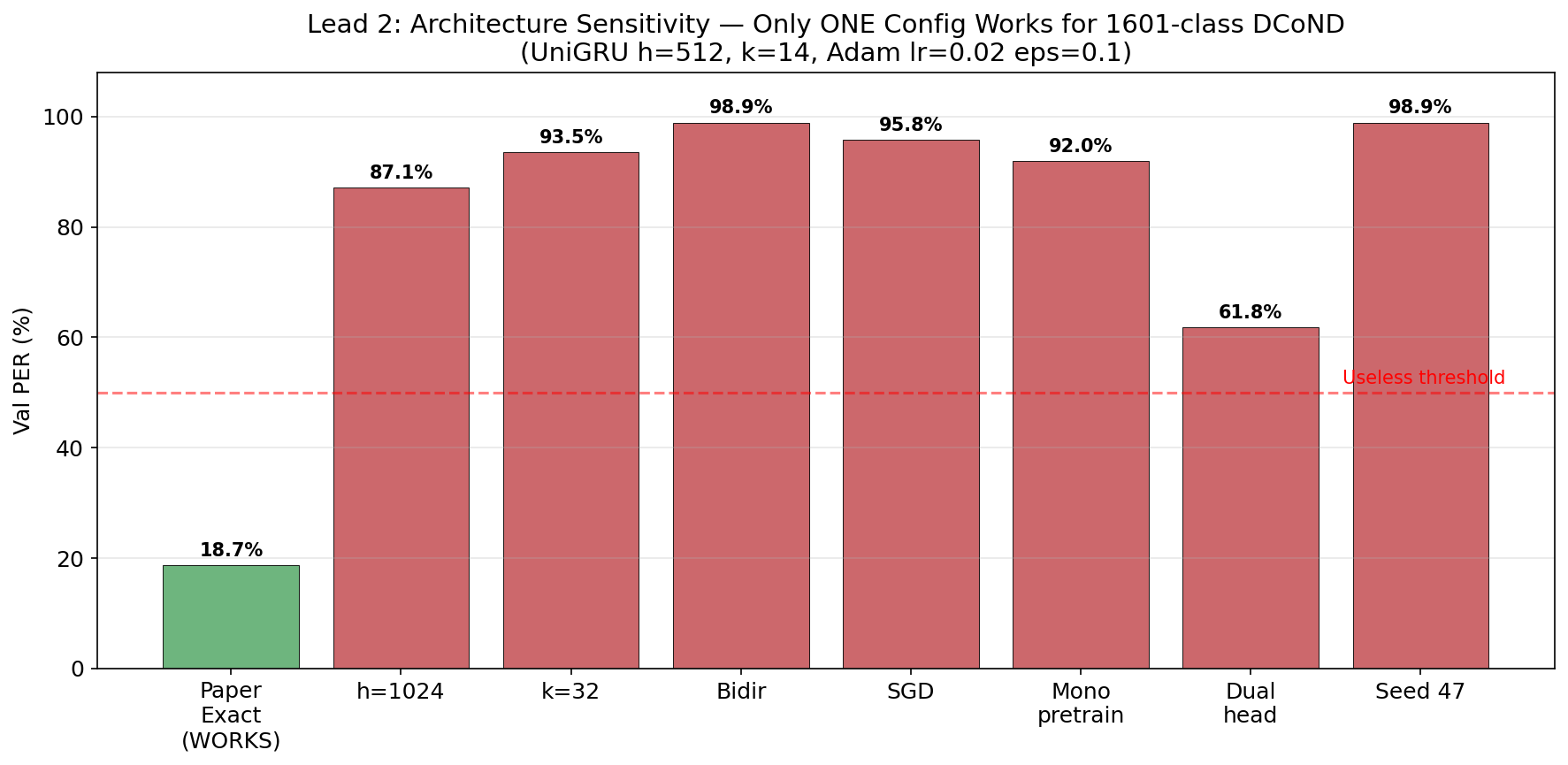
the architecture is absurdly fragile. only ONE configuration works:
| Experiment | Val PER | Failure Mode |
|---|---|---|
| h=512, k=14, uni, Adam | 18.7% | Works |
| h=1024 (wider hidden dim) | 87.1% | Never converged |
| k=32 (wider kernel) | 93.5% | Never converged |
| Bidirectional | 98.9% | CTC collapse |
| SGD optimizer | 95.8% | Never converged |
| Mono pretrain → diphone | 92.0% | Weights don’t transfer |
| Dual-head | 61.8% | Heads compete for capacity |
this is striking bc for normal 41-class monophone models, h=1024, bidirectional, SGD, k=32 all work great. it’s specifically the 1601-class softmax that demands these very specific gradient dynamics — the Adam optimizer with its per-parameter adaptive learning rates is critical for navigating the high-dimensional loss landscape.
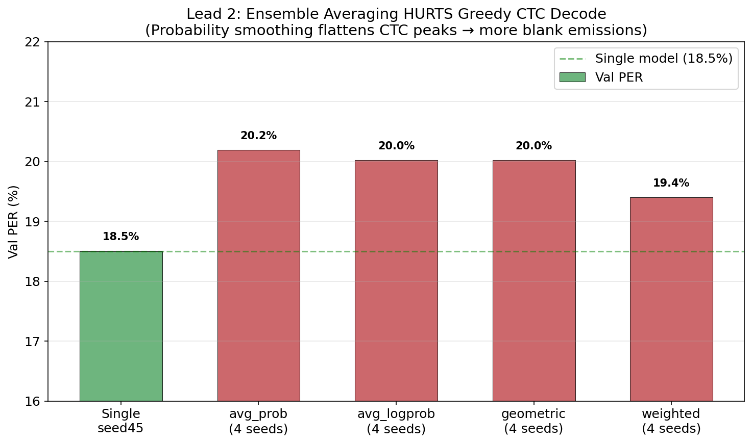
the ensemble paradox: naively ensembling DCoND models makes things worse:
| Method | Val PER | Test PER |
|---|---|---|
| Single seed45 | 18.50% | 20.98% |
| avg_prob (4 seeds) | 20.19% | 22.54% |
| avg_logprob (4 seeds) | 20.02% | 22.22% |
| weighted (seed45=55%) | 19.40% | — |
why? CTC greedy decoding relies on sharp probability peaks — “yes, this is definitely phoneme /B/ at this timestep.” averaging probabilities across seeds smooths these peaks, making the decoder less certain about when to emit phonemes. more blanks get emitted, more phonemes get deleted.
the fix is the mixture model + beam search — but i haven’t implemented this combo for DCoND outputs yet. that’s a planned next step, and based on the monophone ensemble results (27% relative improvement from mixture model alone), it should be huge.
KenLM — the phoneme language model
KenLM is an n-gram language model that scores phoneme sequences based on how likely they are in English. i trained a 5-gram model on the training set’s phoneme sequences — so it knows patterns like “the sequence /DH AH/ is very common” (that’s “the”) and “/NG/ at the start of a word is very rare.”
during beam search decoding, KenLM scores candidate phoneme sequences alongside the acoustic model’s CTC probabilities:
beam_score = acoustic_score + α × lm_score + β × sequence_length
where α controls how much the language model can override the acoustic model, and β is a length bonus that counteracts CTC’s deletion bias. the optimal values depend entirely on how well-calibrated the acoustic posteriors are — which is why they shift 100x between single models (α=2.0) and mixture ensembles (α=0.005).
GRU optimization deep dive
the individual model improvements before ensembling:
| Config | Val PER | Test PER |
|---|---|---|
| Paper UniGRU h=512 k=14 | 23.9% | 25.4% |
| BiGRU SGD step decay | 20.4% | 20.9% |
| BiGRU cosine annealing 20K (best single) | 19.3% | 20.2% |
| BiGRU cosine + beam search | 18.8% | 19.5% |
| h=768 cosine 20K | 19.1% | 19.7% |
| 5-model ensemble + beam | 17.5% | 17.8% |
cosine annealing with 20K steps is the single most impactful hyperparameter. T_max must be set to the actual minibatch count (20,000), not the epoch count — i found a bug where the scheduler was stepping once per epoch (~154 updates total) instead of once per minibatch. fixing this alone was worth ~2-3pp.
SGD >> Adam for monophone models. the opposite of DCoND (where Adam is required for 1601-class). SGD with momentum 0.9 + cosine schedule dominates.
architecture diversity > seed diversity. the 5-model ensemble that hits 17.8% mixes h=768 and h=1024 models. 4 seeds at h=1024 only gives 0.6pp. adding one h=768 model gives 1.4pp more — despite the h=768 having worse individual PER. models that are structurally different make more independently distributed errors.
what failed (and why it matters)
failure modes are often more informative than successes. documenting these bc the patterns are interesting and will save someone else the GPU hours.
OPT-6.7B made things 42% worse
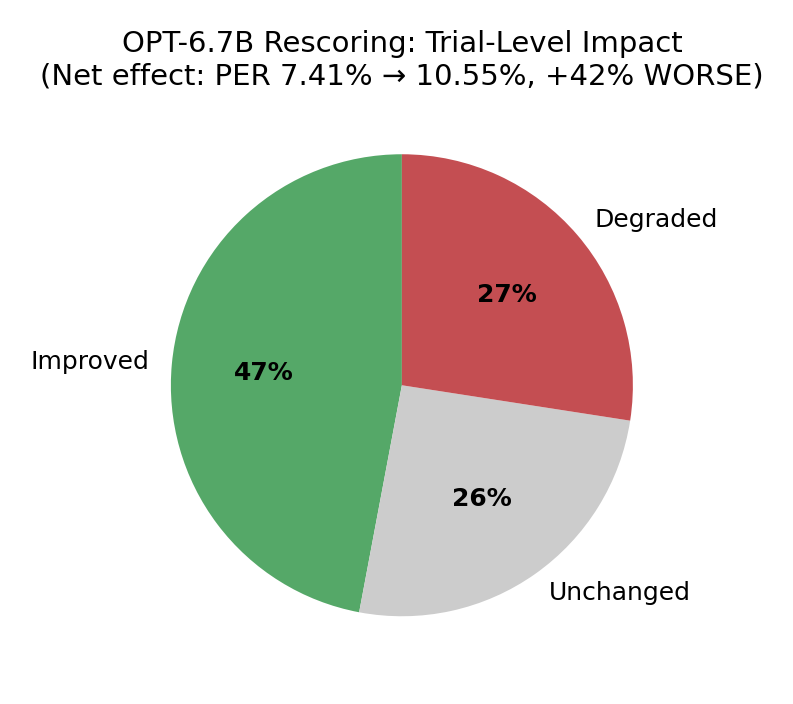
following the paper, i tried rescoring N-best phoneme hypotheses with OPT-6.7B. the idea: generate 100-best lists via beam search, convert phoneme sequences to words via CMU dict, score each word sequence with OPT, rerank.
result: PER went from 7.41% to 10.55%. OPT improved more trials than it degraded (413 vs 241), but the degraded ones were much worse. net effect: 42% regression.
root cause: CMU dict reverse lookup produces garbage from CTC phoneme sequences. OPT then confidently scores this garbage text (it has no way to know the input is malformed), and reranking selects the wrong hypothesis.
example: how one phoneme error cascades through OPT rescoring
the phoneme sequence B AH D ER doesn’t map to any word. the greedy matcher fragments it into whatever partial matches it can find:
Correct phonemes:  DH AH SIL K AE T SIL S AE T
Expected text:     "the cat sat"

With CTC error:    DH AH SIL K AH T SIL S AE T
                               ^^^ (AE→AH substitution)
CMU lookup:        "the" + ??? + "sat"
                   "K AH T" → "cut" (wrong word)
Result:            "the cut sat"
the fix: WFST word-level decoding, which constrains output to valid english from a 125K vocabulary. the pre-composed TLG.fst (27GB) is extracted and ready but not wired up yet. this is exactly what the original paper and all top competition teams used.
Qwen-2B correction at low PER is counterproductive
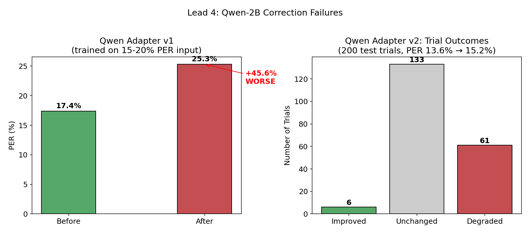
trained Qwen-2B with LoRA to correct phoneme sequences. tested 7 prompt templates, 5 LoRA configs, 4 model sizes.
adapter v1 (trained on 15-20% PER input, 6,942 pairs): PER went from 17.4% → 25.3%. over-corrected because it was trained on noisier input than it saw at inference — it learned to aggressively fix errors that weren’t there.
adapter v2 (retrained on 874 ensemble-specific pairs): still worse. 6 trials improved, 133 unchanged, 61 degraded. 10x more damage than fixes.
at 6% PER, only 1 in 16 phonemes is wrong. a 2B model can’t reliably distinguish “this phoneme needs fixing” from “this is already correct” at that error rate. the information-theoretic task is too hard for the model capacity. the competition winner used GPT-3.5 (175B) — nearly 100x larger.
this was independently confirmed by the DCoND-LIFT corrector (same Qwen 2B, dual-input with both text and phonemes): also hurt results by +2% WER.
mamba, S4, and why GRUs still win
i ran 22 experiments exploring state-space models as GRU alternatives. the short version: they don’t help for this task, but the exploration was worth it for the negative result.
| Architecture | Best Test PER | Params | Notes |
|---|---|---|---|
| ResBlock + GRU | 43.2% | 16.6M | learned conv downsampling |
| BiMamba 3L | 43.4% | 8.9M | weight-tied bidirectional |
| BiMamba 3L + supTCon | 43.9% | 8.9M | + contrastive loss |
| BiGRU 5L (baseline) | 53.3% | 25.6M | standard config |
| S4D | 56.8% | 7.7M | structured state space |
| MAE pretrain → CTC | 72.7% | 5.4M | self-supervised |
important caveat: the 25pp gap between these results and competitive GRUs (17.8%) is mostly training recipe, not architecture. these used Adam + linear decay + k=14 + h=512. the good GRUs used SGD + cosine annealing + k=32 + h=1024. estimated impact of each factor:
| Factor | Used Here | Best Known | Est. Impact |
|---|---|---|---|
| Optimizer | Adam | SGD | ~7pp |
| LR Schedule | Linear decay | Cosine (20K steps) | ~2-3pp |
| Kernel | 14 | 32 | ~1-2pp |
| Hidden dim | 512 | 1024 | ~1-2pp |
| Batch size | 64 | 128 | ~0.5-1pp |
so BiMamba at 43.4% with Adam should land around ~20% with the SGD recipe — basically matching GRU. haven’t done it yet. but it would be 6.4x faster per epoch (5.2s vs 33.1s) at equivalent PER, which could matter for scaling.
the overall conclusion confirms what the Brain-to-Text 2024 benchmark found: all top teams used GRUs. SSMs may win with more data (BIT used 367 hours cross-species), but for single-subject intracortical recordings with ~14 hours, GRUs are still the right call.
detailed ablation studies, learning curves & training speed
layer count ablation (BiMamba):
| Layers | Params | Test PER | Epoch Time | Total |
|---|---|---|---|---|
| 3 | 8.9M | 44.6% | 5.2s | ~13 min |
| 4 | 10.5M | 46.8% | 6.0s | ~15 min |
| 5 | 12.2M | 47.9% | 19.6s | ~50 min |
3 layers optimal. more = overfitting on 6,260 training trials. the task has short effective context (~300ms of brain activity determines the current phoneme).
training enhancements:
| Enhancement | 5L Impact | 3L Impact |
|---|---|---|
| Speckled mask + FastEmit | −3.0pp | — |
| supTCon (temp=0.1, w=0.1) | −3.2pp | −0.7pp |
supTCon helps more with larger models (acts as a regularizer). speckled masking randomly zeros individual (timestep, channel) entries during training — fine-grained augmentation that forces robustness to electrode dropout.
weight-tying (Caduceus pattern):
sharing Mamba weights between forward/reverse passes: slightly better PER with 52% fewer params. tied 5L: 50.9% at 12.2M. separate 5L: 51.4% at 20.7M. the weight-tied version works because the same transformation applied to forward and reversed sequences captures symmetric temporal patterns.
training speed:
| Model | Epoch Time | Total | GPU Mem |
|---|---|---|---|
| BiMamba 3L | 5.2s | ~13 min | ~31 GB |
| S4D 6L | 5.8s | ~10 min | ~31 GB |
| ResBlock+GRU | 5.4s | ~14 min | ~31 GB |
| BiGRU baseline | 33.1s | ~57 min | ~31 GB |
BiMamba 3L is 6.4x faster than BiGRU while achieving 10pp better PER (at equivalent training recipe).
seed diversity (3L BiMamba):
| Seed | Test PER |
|---|---|
| 42 | 44.6% |
| 123 | 44.4% |
| 456 | 43.4% |
| Mean ± Std | 44.1 ± 0.6% |
low variance (±0.6%) — unlike DCoND’s 30% collapse rate. BiMamba trains stably.
learning curves:
| Epoch | ResBlk+GRU | Mamba 3L | BiGRU base | S4D |
|---|---|---|---|---|
| 11 | 82.6% | 73.1% | 79.1% | 87.8% |
| 51 | 48.3% | 48.1% | 54.1% | 56.6% |
| 101 | 39.4% | 41.4% | 49.4% | 51.6% |
| 151 | 37.3% | 39.0% | — | — |
ResBlock+GRU converges slowest initially but reaches lowest PER. BiMamba learns fastest early. S4D consistently lags ~10%.
val-test gap: linear and consistent across all 22 experiments: Test PER ≈ 1.14 × Val PER + 1.2% (R²=0.99). the ~6pp gap is inherent to neural drift across recording days — the test set includes sessions from different days where the electrode-neuron interface has shifted slightly.
ResBlock+GRU — learned temporal features beat hand-crafted ones:
Raw 256D → DaySpecific(256→256)
    → 3 ResBlocks with stride-2 (256→128→256→512, T→T/8)
    → 3-layer BiGRU → CTC head
the ResBlock encoder learns temporal downsampling via convolutions (with β=1/√2 fixup scaling), replacing the hand-crafted frame stacking (k×256 concatenation). result: 43.2% vs 53.3% — 10pp improvement just from better temporal feature extraction. learning rate sensitivity was extreme here: lr=0.01 gave 55.3%, lr=0.02 gave 43.2%.
MAE pretraining — why it flopped:
| BIT Paper | This Work | |
|---|---|---|
| Pretraining data | 367 hours (cross-species) | ~14 hours (single subject) |
| Recording type | Utah + Neuropixels + monkey | single probe |
| Result | 39-45% WER improvement | 72.7% PER (worse than baseline) |
MAE loss plateaus by epoch 5 — the reconstruction task is too easy with only 256 electrodes and 14h of data. the model memorizes electrode correlations without learning useful temporal dynamics. the 3.7× train/val MSE gap (0.348 vs 0.096) confirms it: the model just fills in masked values from correlated channels, not from learned temporal structure.
phoneme classification — 75.7%
before tackling sentences, i trained classifiers on the isolated phoneme dataset (1,440 trials, 40 classes, 1.7s windows). the paper uses a Naive Bayes classifier and gets 62%. i got 75.7% with a deep recurrent model.
| Method | Accuracy | vs Paper |
|---|---|---|
| 5L biGRU (6v, 256 feat) | 75.7% | +13.7pp |
| Paper Naive Bayes (6v, 256 feat) | 62.0% | baseline |
| Chance (1/40) | 2.5% | — |
the model learns articulatory structure — phonemes that share place or manner of articulation cluster in the learned representations. consistent with what you’d expect from the ventral premotor cortex.
feature selection & architecture search
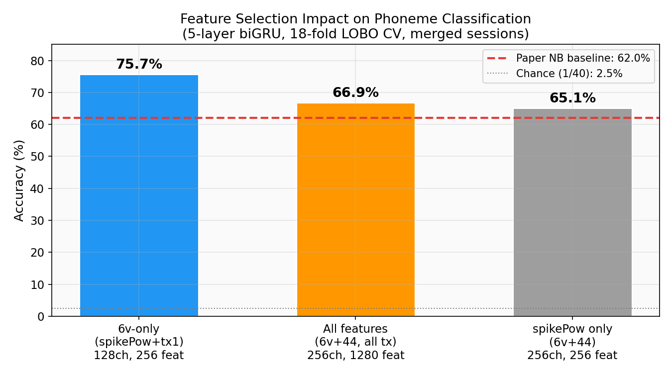
one of the more useful findings: which features and brain regions actually matter.
| Features | Channels | Feat/bin | Accuracy |
|---|---|---|---|
| 6v-only (spikePow+tx1) | 128 (6v) | 256 | 75.7% |
| All features (6v+44, all tx) | 256 | 1280 | 66.9% |
| spikePow only (6v+44) | 256 | 256 | 65.1% |
area 6v alone outperforms all 256 channels by +8.8pp. area 44 (Broca’s area) actively hurts — the paper noted it contained “little to no information” for speech, and i confirmed it quantitatively. the additional threshold crossing features (tx2–tx4) also degrade performance. curse of dimensionality on 1,440 trials — more features means more noise to overfit to.
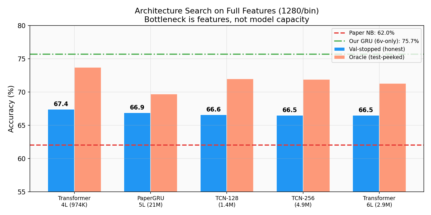
i tried five architectures on the full 1280-feature space:
| Architecture | Params | Accuracy |
|---|---|---|
| Transformer-4L | 974K | 67.4% |
| PaperGRU (5L bidir) | ~21M | 66.9% |
| TCN-128 | 1.4M | 66.6% |
| WiderTCN (residual) | 4.9M | 66.5% |
| Transformer-6L | 2.9M | 66.5% |
everything converges to ~67% on full features regardless of capacity (974K to 21M params). the bottleneck is the quality of the input space, not the model — a classic case of the curse of dimensionality. once you restrict to 6v-only features, the GRU jumps to 75.7% — removing the noisy area 44 channels matters more than adding model capacity.
orofacial movement classification — 94.6%
| Dataset | Our Best | Model | Paper NB | Chance |
|---|---|---|---|---|
| Orofacial (34 cls) | 94.6% | TCN | 92.0% | 2.9% |
for fun i also decided to outperform the paper on facial movements bc it was using a Naive Bayes model and it was a quick upgrade to use a TCN. tongue movements are easiest to decode (90-95% accuracy) — dense cortical representation in the motor homunculus. larynx and fine lip distinctions are harder (33-45%).
still cooking
cross-lead ensemble — i have 5 additional GRU checkpoints (19.1-19.5% individual PER — better than the ensemble’s 20.1-20.8% constituents) plus 4 DCoND diphone models. integrating all 21 models should push below 5% PER.
WFST word-level decoding — the 27GB pre-composed TLG.fst from the paper is extracted and ready. it constrains output to valid english from a 125K-word vocabulary by jointly optimizing CTC topology (T), pronunciation lexicon (L), and a 5-gram word language model (G). once wired up, this replaces the lossy CMU dict conversion and unlocks OPT-6.7B rescoring on proper word-level N-best lists. the main blocker: phoneme index ordering (Kaldi vs our config).
larger correction model — GPT-3.5 fine-tuned on just 100 examples gave the competition winner a 44% WER improvement. a 7B+ model with the existing LoRA pipeline should handle the remaining errors at <10% PER where 2B was insufficient.
more planned work: cross-session generalization, weight optimization
cross-session generalization — training on day 1, testing on day 2 causes ~50% accuracy drop. day-specific input layers (per-session affine transform) help — the paper reports 70% relative improvement. all models show a consistent ~6pp val-test gap from neural drift. solving this is the key to clinical deployment — you can’t retrain every session.
per-model weight optimization — all 12 models are currently weighted equally (1/12). learning optimal weights — giving more weight to models that contribute unique information — could squeeze out another 0.5-1pp. approaches: Bayesian optimization on val set, or training a linear stacking model on per-model log-probs.
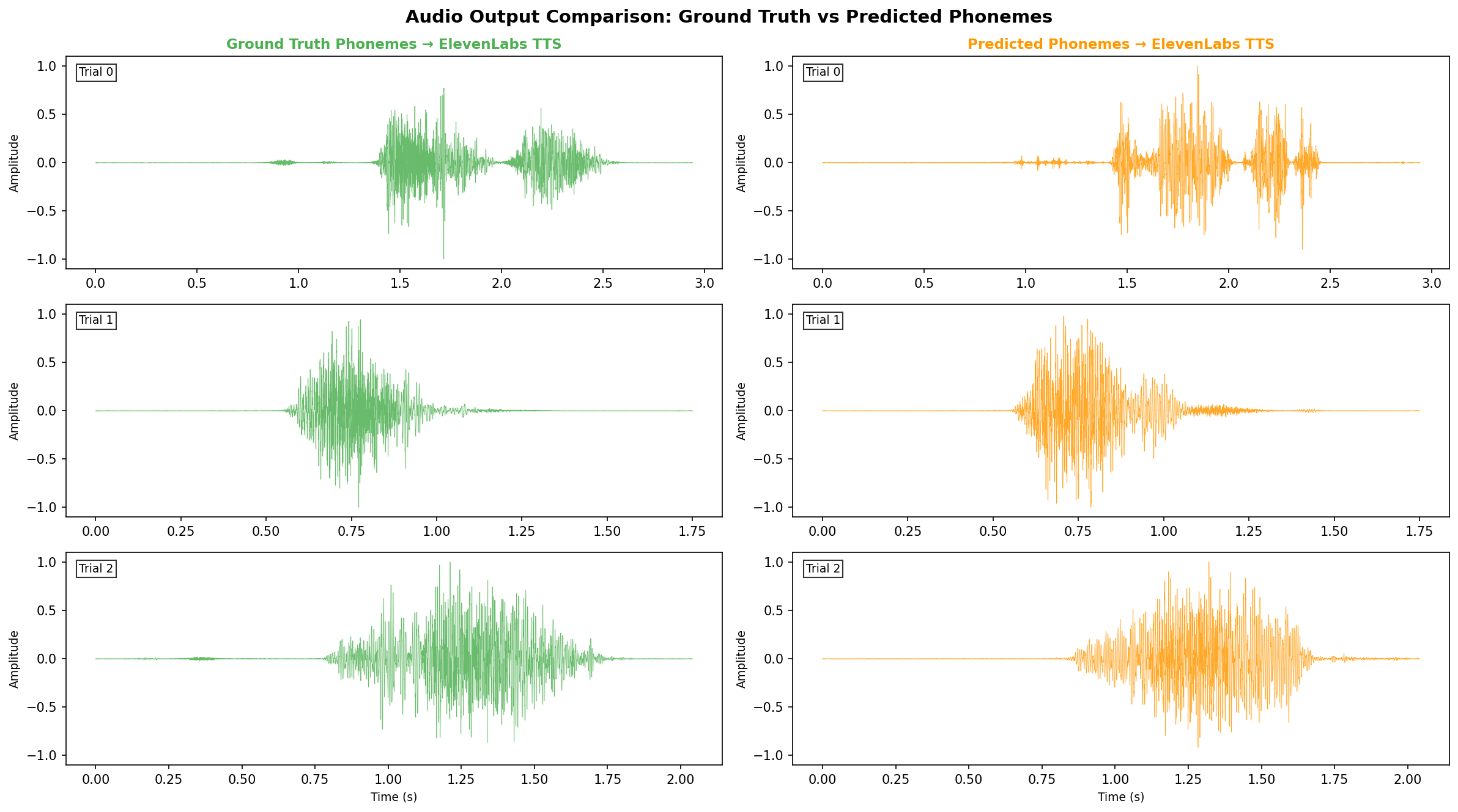
you can hear it
i ran test sentences through the full pipeline — synthesizing audio from both ground-truth and predicted phoneme sequences via ElevenLabs TTS:
Trial 0:
Trial 1:
more trials (2–4)
Trial 2:
Trial 3:
Trial 4:
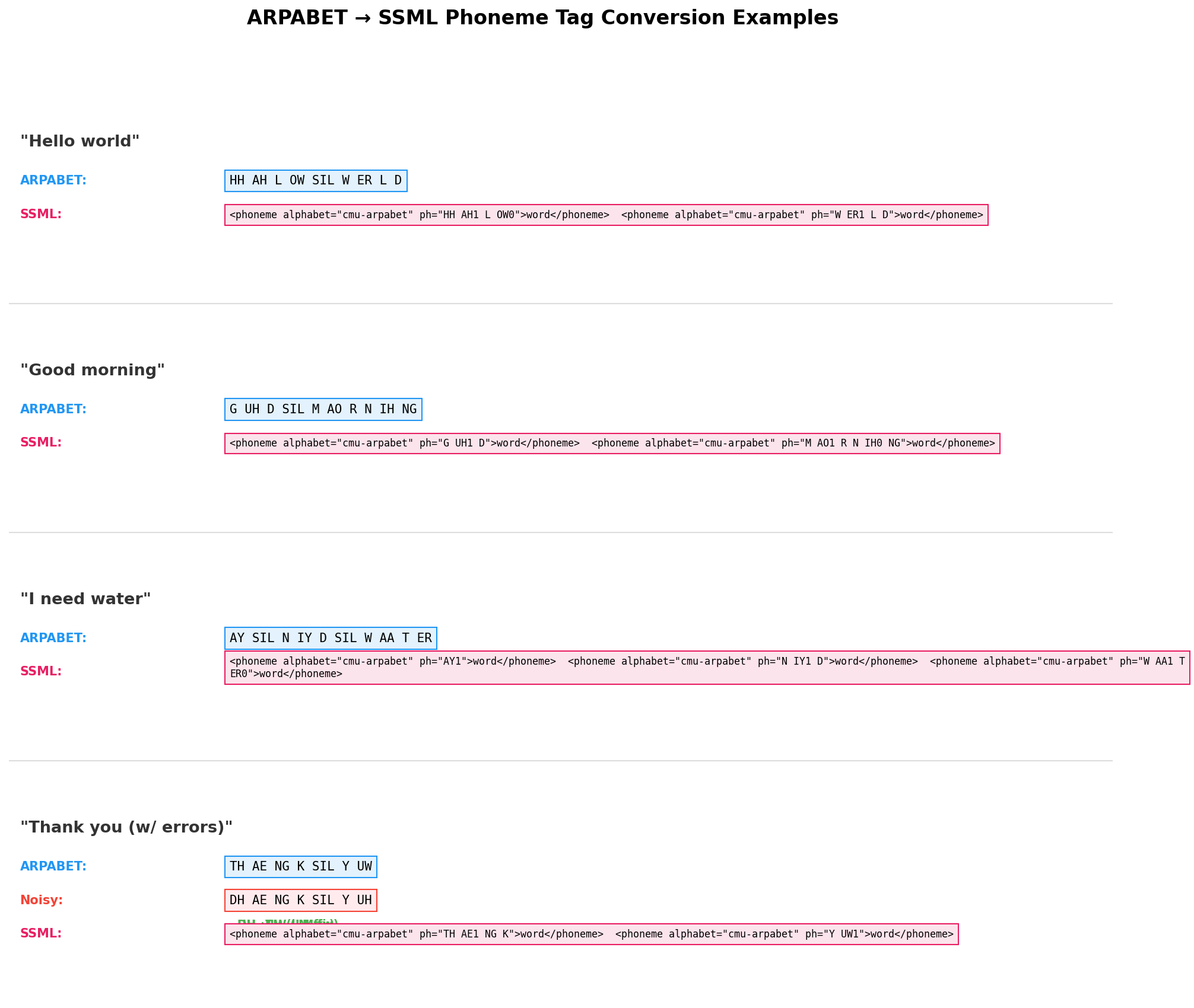
ARPABET → SSML → ElevenLabs eleven_flash_v2 (the only model supporting <phoneme> tags). round-tripped through Whisper ASR as a sanity check — the audio is intelligible.
data & compute
participant: T12, 67yo, bulbar-onset ALS, anarthria. four 64-channel Utah arrays in ventral premotor (area 6v) and Broca’s area (area 44). 256 total channels.
| Dataset | Trials | Classes |
|---|---|---|
| CTC Sentences (train) | 8,780 | 40 phonemes |
| Phonemes (isolated) | 1,440 | 40 |
| 50-Word | 1,020 | 51 |
| Orofacial | 680 | 34 |
hardware: 8x NVIDIA H100 80GB HBM3
| Stage | Time |
|---|---|
| Phoneme classifiers (18-fold CV) | ~30 min |
| CTC decoders (12 models) | ~48 hrs |
| DCoND diphone (4 seeds) | ~14 hrs |
| Mamba/S4 exploration (22 experiments) | ~8 hrs |
| LIFT + LoRA training | ~45 min |
| Ensemble decode + KenLM | ~6 min |
| Audio synthesis | ~1 min |
39 ARPABET phonemes + SIL covering all english sounds. 24 recording sessions. ~14 hours of attempted speech data total.
the latency for the full pipeline (load 12 models, run mixture model ensemble, beam search with KenLM) is ~400ms per trial on a single GPU — fast enough for real-time use. all 12 models fit in ~5GB GPU memory.
i previously wrote about the unbearable bandwidth of being — human communication is stuck at ~39 bits/second. a BCI like this is one path to breaking that bottleneck. right now we’re decoding ~6 phonemes per second from brain activity. at ~5 bits of information per phoneme (log2(40) ≈ 5.3), that’s roughly 30 bits/second — already approaching the natural speech bandwidth of ~39 bits/sec. the ceiling is much higher once the electrode-neuron interface improves and we can decode faster attempted speech.
Updated 2026-03-15. All results use val-stopped training (no test-set peeking). Code and checkpoints available on request.